
Wind Power Curve Calibration
Calibration of Renewables Power Curves
Section titled “Calibration of Renewables Power Curves”| Concept | Description |
|---|---|
| Objective | Produce realistic and localised generation forecasts monthly |
| Scope | Calibrating power curves for individual generators - modelling the relationship between historical climate data at their location and observed electricity generation to estimate future output |
| Why approach chosen | Historical data is used because long-term climate conditions and seasonal trends are generally stable, offering a dependable foundation for estimating monthly electricity generation |
| What feeds this | ELFO’s generation forecast, Scheme Valuation Model |
| Time horizon | Trained on data from 1980 to present, project load factors for future years (currently up to 2050) |
Context
Section titled “Context”Often we represent plant generation as a load factor, which is derived by dividing generation data by the plant’s maximum contract capacity. We have data on generation since the start of a CfD contract. We also know what GB weather conditions were in specific locations going all the way back to 1980 based on ERA5 data (ERA5 hourly data on single levels). Using these two sources, we model the relationship between historical load factors for our plants and observed weather conditions. This process produces a power curve function, which we can then use to estimate the load factor of a wind plant based on its wind speed data inputs, or estimate the load factor of a solar plant based on its temperature and radiation data inputs.
This page explains the reasoning and theories followed to calibrate power curves. Once the newly calibrated power curves have been obtained, they can be used to estimate future electricity generation. In case actual data are not yet available for a specific generator, default parameter can be used to estimate the generation.
Output Sample
Section titled “Output Sample”| PLANT ID | a | b | c | d | g | Estimated Load Factor |
|---|---|---|---|---|---|---|
| AAA-ACH-183 | 0 | 3.6792376 | 14.142865 | 1 | 2.7610703 | 0.334300011 |
| AAA-BAD-185 | 0 | 5.556794 | 6.4739075 | 1 | 0.26575124 | 0.311800003 |
| AAA-BAN-189 | 0 | 5.665352 | 4.973238 | 1 | 0.16442393 | 0.245299995 |
| AAA-BAN-192 | 0 | 6.5032425 | 5.2156076 | 1 | 0.13102184 | 0.222100005 |
| AAA-COI-196 | 0 | 2.724648 | 13.884499 | 1 | 2.5957184 | 0.252400011 |
| AAA-DOR-182 | 0 | 22.520182 | 1.9434453 | 1 | 0.00867856 | 0.181400001 |
| AAA-NAN-184 | 0 | 5.2470207 | 2.6030238 | 1 | 0.10859738 | 0.317600012 |
| AAA-NEA-195 | 0 | 14.838868 | 3.5576274 | 1 | 0.0151439 | 0.1523 |
| AAA-PNE-187 | 0 | 3.7041304 | 11.440603 | 1 | 1.4981503 | 0.313899994 |
| AAA-SOL-181 | 0 | 4.381013 | 6.134548 | 1 | 0.44254097 | 0.305900007 |
| AR2-HRN-106 | 0 | 4.615351 | 9.434262 | 1 | 0.8291254 | 0.423200011 |
| AR2-HRN-206 | 0 | 4.634624 | 9.61741 | 1 | 0.92562836 | 0.434100002 |
| AR2-HRN-306 | 0 | 4.8454447 | 8.631197 | 1 | 0.65937406 | 0.429100007 |
| AR2-MRY-107 | 0 | 17.036682 | 3.0932243 | 1 | 0.01531285 | 0.215000004 |
| AR2-MRY-207 | 0 | 19.927872 | 3.2953153 | 1 | 0.01365842 | 0.214900002 |
| AR2-MRY-307 | 0 | 17.025848 | 3.0932193 | 1 | 0.01532271 | 0.215000004 |
| AR2-TKN-103 | 0 | 5.0062895 | 9.416339 | 1 | 0.8114719 | 0.393599987 |
| AR2-TKN-203 | 0 | 5.0061398 | 9.416673 | 1 | 0.81155443 | 0.393599987 |
| AR2-TKN-303 | 0 | 4.8241396 | 9.756517 | 1 | 0.85578257 | 0.393000007 |
| AR4-BCW-610 | 0 | 12.28112 | 3.1404097 | 1 | 0.01654289 | 0.134000003 |
| AR4-HHR-610 | 0 | 5.088788 | 6.6896195 | 1 | 0.14213328 | 0.1215 |
| CAA-EAS-166 | 0 | 4.7525225 | 9.136884 | 1 | 0.89301986 | 0.446399987 |
| CAA-EAS-167 | 0 | 4.7524548 | 9.137065 | 1 | 0.8930717 | 0.446399987 |
| CAA-EAS-168 | 0 | 4.752557 | 9.136933 | 1 | 0.8930427 | 0.446399987 |
| INV-BEA-001 | 0 | 5.6598573 | 7.3345356 | 1 | 0.39816892 | 0.388099998 |
| INV-BEA-002 | 0 | 4.8215337 | 8.914363 | 1 | 0.67768973 | 0.393900007 |
| INV-BUR-001 | 0 | 4.2666755 | 10.2099695 | 1 | 1.5506972 | 0.38409999 |
| INV-DUD-001 | 0 | 4.473937 | 11.379135 | 1 | 1.8926902 | 0.45480001 |
| INV-DUD-002 | 0 | 3.8923666 | 29.909513 | 1 | 61.087887 | 0.469700009 |
| INV-DUD-003 | 0 | 4.1432033 | 14.048186 | 1 | 4.0743523 | 0.469500005 |
| INV-HOR-001 | 0 | 4.9800014 | 9.099786 | 1 | 0.8686544 | 0.459600002 |
| INV-HOR-002 | 0 | 4.841342 | 8.316067 | 1 | 0.65941435 | 0.452699989 |
| INV-HOR-003 | 0 | 4.795151 | 9.79731 | 1 | 1.0198916 | 0.444000006 |
| INV-WAL-001 | 0 | 4.9462557 | 8.25572 | 1 | 0.63509107 | 0.425300002 |
| INV-WAL-002 | 0 | 3.8824124 | 14.502575 | 1 | 3.926563 | 0.451999992 |
| Generic Offshore Wind | 0 | 8.07483 | 8.854368 | 1 | 3.6699734 | 0 |
| Generic Onshore Wind | 0 | 7.283319 | 6.653677 | 1 | 0.6801953 | 0 |
This is a sample output from the calibration summary, which contains the logistic function parameters for each calibrated plant. It also reports an estimated long-term load factor which is based on the historical distribution of wind speeds for the plant location. At the bottom of the file, generic curve parameters are reported for both onshore and offshore wind, which can be used for uncalibrated plants. Note that these have their estimated load factor at 0 as there is no knowledge of localised wind speed distributions.
Wind Power Curve
Section titled “Wind Power Curve”Three activities need to be carried out to calculate the parameters and produce the load factor stream:
- Update the ERA5 data to obtain the latest historical wind data for GB
- Calibrate the wind power curve for each CfD generator, based on actual data where available
- Create the individual wind streams from the historic data with specific information for CFD generators in GB
To calibrate the power curve for the CFD wind farm the following data are needed:
- Actual hourly load factor data (generation/capacity) for a significant time interval.
- Hourly actual wind speed data for the closest available location (from ERA5 dataset) for the same period the actual load factors data are available.
Wind calibration in rencal uses two model components:
- a logistic power curve to map wind speed to expected load factor;
- a Weibull wind-speed distribution to describe how frequently wind speeds occur at each plant location.
Among available models for plant output conversion, the five-parameter logistic function (5PL) has been chosen because it combines a single analytical expression with good empirical fit once calibrated. For deeper mathematical detail, see Logistic Power Curve.
The Weibull component is then used with the logistic curve to estimate long-term expected load factor by probability-weighting wind speeds. For details, see Weibull Wind-Speed Distribution.
To use the 5PL function to forecast wind energy output it is necessary beforehand to define the five parameters through a calibration process run over actual wind speed and generation data.
The definition of the parameters is accomplished through a least square regression to find the power curve that fits best the actual data, allowing to calculate the best fit parameters a, b, c, d and g that minimize the error on the load factor.
After the determination of the five parameters, the analytical function can be easily applied to a forecast hourly wind speed dataset to evaluate the corresponding hourly load factor.
Practically what this process means is we can use the power curve to produce historical estimates (i.e. backcast), obtaining estimated load factors for plant locations back to 1980, as well as future estimates. Outputs from this process produce hourly load factors for each generator (aka wind streams).
Calibrated vs. Default
Section titled “Calibrated vs. Default”With newly operational plants, quite often we have minimal historical generation for which to derive a plant specific forecast. In other words, we don’t have enough generation data to confidently derive a power curve function, which can then be used to estimate historical values. In these instances, a generic power curve would be applied to the wind speeds at the location of the plant to generate wind streams.
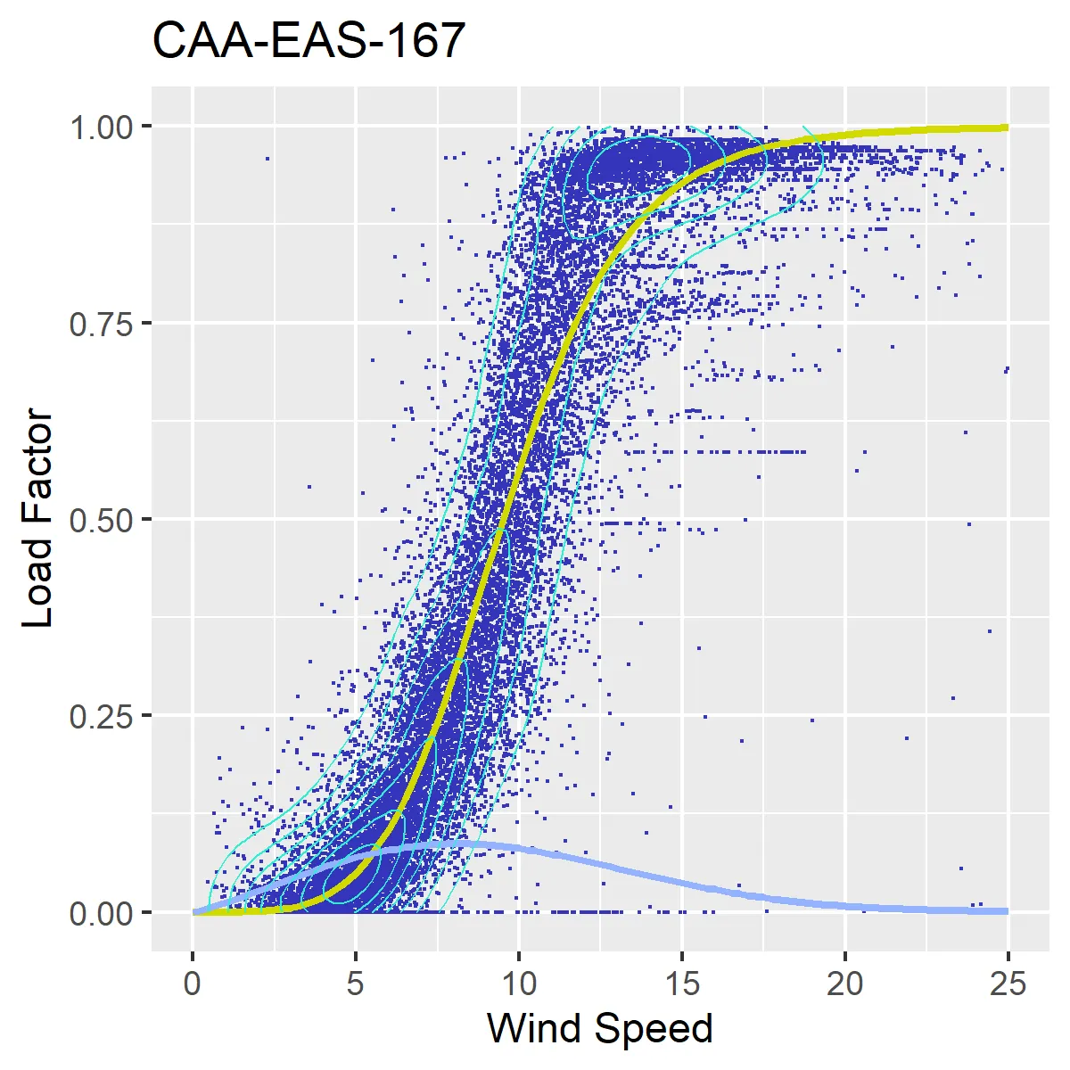
By applying analytical judgement and looking at the individual CFD units’ plots, one can determine which CFDs have produced a power curve that closely approximate the actual data and is hence acceptable to be used in the forecasting process. A default power curve should be used for generators whose calibration is not suitable.
e.g. model (yellow line) below approximates the actual data (blue dots).