

Logistic Power Curve
Logistic Power Curve
Section titled “Logistic Power Curve”Context
Section titled “Context”In wind calibration, the logistic power curve models how expected plant load factor changes as wind speed increases.
It gives us a compact analytical expression that can be fitted to historical observations and then reused to convert hourly wind speed into hourly load factor.
Generalised Logistic Function (5PL)
Section titled “Generalised Logistic Function (5PL)”The general form is:
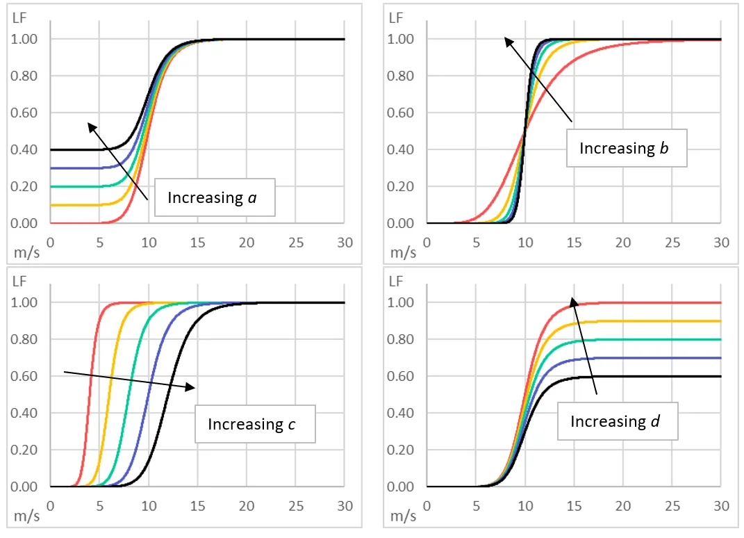
Parameter interpretation:
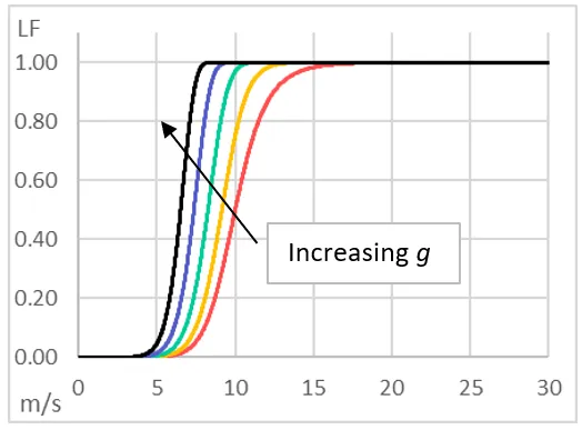
a: lower bound (minimum production)b: slope/steepnessc: inflection pointd: upper bound (maximum production)g: asymmetry factor (g = 1gives a symmetric shape)
For wind load factors in this workflow, bounds are fixed to:
a = 0d = 1
So the fitted shape parameters are effectively b, c, and g.
Why this model is used
Section titled “Why this model is used”- Single analytical expression, easy to evaluate at scale.
- Flexible enough to represent the S-shaped response of wind output.
- Fitted directly to historical plant data via least-squares calibration.
How it is used in rencal
Section titled “How it is used in rencal”- Implemented in
WindCalibrator.logistic_function(). - Fitted as part of calibration flow in
WindCalibrator.estimate_load_factors_for_resource(). - Applied hour-by-hour to wind speed data to produce
Wind Streams.parquet.